Understanding Bayesian Inference: Linear Regression

From Seed Germination to Tree Improvement to Business Decisions

When in doubt, just fit straight lines. ;P

Introduction

In our previous post, we explored the foundations of Bayesian inference through a simple example: estimating germination rates from seed trials. We learned how to specify priors, update beliefs with data through Bayes’ theorem, and make probabilistic predictions. The key insight was treating parameters as random variables with probability distributions, allowing us to make direct statements like “there’s a 95% probability the germination rate is between 0.42 and 0.75.”

That example involved estimating a single parameter – a probability $\theta$. The Beta-Binomial model was simple: one probability to estimate, one prior to specify. But most real-world problems involve relationships between variables: How does tree height relate to diameter? How does drug dosage affect blood pressure? How do temperature and rainfall predict crop yield? These questions require regression models with multiple parameters: slopes, intercepts, and error terms.

You might be wondering: does Bayesian inference scale to more complex problems? What happens when we have multiple parameters that interact?

The answer is both simple and profound: the logic doesn’t change at all. Whether you have 1 parameter or 100, the Bayesian workflow remains identical. You specify priors for each parameter, observe data, apply Bayes’ theorem, and make predictions. The mathematics gets more complex, but the conceptual framework is exactly the same.

This post demonstrates that claim by extending everything you learned about seed germination to linear regression with multiple predictors. We’ll work through two examples:

• Example 1: Predicting tree height from diameter – learning why prior choice matters
• Example 2: Evaluating tree improvement programs – making economic decisions with uncertainty

By the end, you’ll see that if you understood how to update beliefs about germination rates, you already understand Bayesian regression – we’re just working with more parameters simultaneously.

A Brief Historical Note: Francis Galton and the Origins of Regression

Before diving into our analysis, it’s worth appreciating where linear regression came from. The method we’re about to use has a fascinating origin story rooted in Victorian-era genetics and an obsession with heredity.

Sir Francis Galton (1822-1911), a polymath and Charles Darwin’s half-cousin, pioneered regression while studying inheritance patterns. In the 1880s, Galton collected data on the heights of parents and their adult children. He discovered something curious: tall parents tended to have tall children (as expected), but those children were, on average, shorter than their parents. Conversely, short parents tended to have children who were taller than them.

Galton called this phenomenon “regression toward mediocrity” – later shortened to simply “regression.” The children’s heights “regressed” toward the population mean. This observation led him to develop the mathematical tools for describing the linear relationship between two variables (Galton, 1886).

The method’s name is now somewhat misleading: Today, when we say “regression,” we’re usually talking about predicting one variable from another using a mathematical equation. We’re not talking about Galton’s original “regression to the mean” phenomenon (where extreme values tend toward average in the next generation).

So how did we end up with this confusing terminology? Galton’s discovery of regression-to-the-mean led him to develop the mathematical tools for fitting straight lines through data. The name “regression” stuck to describe the method (fitting lines), even though we now use that method for all sorts of predictions that have nothing to do with the original “regressing toward mediocrity” concept.

In modern usage: When we fit a regression model to predict tree heights from diameters, we’re using the same linear equation framework that Galton developed—but we’re not studying regression-to-the-mean. We’re simply modeling how one variable relates to another. The historical origin of the name is now just an interesting footnote.

Karl Pearson (1857-1936), Galton’s protégé, formalized these ideas into the regression methods we use today, developing the mathematics of correlation and least squares estimation (Pearson, 1896). Interestingly, while Galton and Pearson developed their methods in a frequentist framework – focusing on best-fit lines through data – the Bayesian approach we’ll use asks slightly different questions: not just “what line best fits this data?” but “given this data, what can we believe about the relationship?”

The tree data we’ll analyze follows Galton’s original spirit: we’re exploring biological relationships where larger individuals tend to have other larger characteristics, though with considerable variation around the trend.

Example 1: A Simple Start - Predicting Tree Height from Diameter

We’ll begin with a straightforward example: predicting tree height from diameter using the classic trees dataset. This single-predictor model will help us understand the Bayesian regression workflow and – crucially – see why prior choice matters.

The Data

library(rstanarm)
library(tidybayes)
library(bayesplot)
library(tidyverse)
library(patchwork)

# Load and prepare data
scale_factor <- 10  # Scale DBH by 10 cm units

# Convert to metric and scale for better interpretation
trees <- datasets::trees %>%
  mutate(
    dbh = Girth * 2.54,                           # inches -> cm
    height = Height * 0.3048,                     # feet -> meters
    volume = Volume * 0.0283168,                  # cubic feet -> cubic meters
    dbh_scaled = (dbh - mean(dbh)) / scale_factor # center and scale by 10 cm
  )

# Quick look at the relationship
ggplot(trees, aes(x = dbh, y = height)) +
  geom_point(size = 3, alpha = 0.7) +
  labs(
    title = "Tree Height vs. Diameter", 
    subtitle = "Black Cherry Trees (n = 31)",
    x = "Diameter at Breast Height (cm)", 
    y = "Height (m)"
  ) +
  theme_minimal()

The relationship looks roughly linear and positive – we expect taller trees to have larger diameters.

The Model

We’ll predict tree height from diameter:

$$\begin{array}{rl}{y}_i& \sim \text{Normal}({\mu }_i,\sigma )\\ {\mu }_i& =\alpha +\beta \cdot x_i\\ \alpha & \sim \text{Normal}(20,3)\\ \beta & \sim \text{Normal}(1,1)\\ \sigma & \sim \text{Exponential}(0.5)\end{array}$$

In words:

• What we’re predicting: $y_i$ is the observed height (in meters) for tree $i$
• The model structure: Each tree’s height comes from a Normal distribution with mean ${\mu }_i$ and standard deviation $\sigma$
• The relationship: Mean height ${\mu }_i$ depends linearly on diameter through $\alpha +\beta \cdot x_i$, where $x_i$ is the scaled diameter (DBH) for tree $i$
• What the priors represent: Our uncertainty about the model parameters before seeing the data
  • $\text{Normal}(20,3)$ for intercept ($\alpha$): expected height at mean DBH is around 20 meters
  • $\text{Normal}(1,1)$ for slope ($\beta$): height increases by roughly 1 meter per 10 cm increase in DBH
  • $\text{Exponential}(0.5)$ for residual standard deviation ($\sigma$): constrains variation to be positive
• Why we scale the diameter predictor: We center DBH (subtract the mean) and divide by 10 cm to make the slope coefficient more interpretable. After scaling, $\beta$ represents “change in height per 10 cm increase in diameter” rather than “per 1 cm increase.” This makes prior specification easier (we can think in meaningful units like “does height increase by ~1 meter per 10 cm of diameter?”) and helps the MCMC sampler run more efficiently.
• Why these priors work: They encode basic domain knowledge (trees are positive heights, larger diameter → taller) while remaining weak enough that the data can easily override them if reality differs

Why Prior Choice Matters: Revisiting a Key Lesson

In our seed germination example, we compared different priors (uniform, weakly informative, and strongly informative) and saw how they updated with data. That example involved a single parameter bounded between 0 and 1, making it relatively straightforward to specify sensible priors.

But regression introduces new challenges: multiple parameters on different scales that interact. This is where the “flat priors are objective” misconception becomes especially dangerous.

Recall from the frequentist post that all statistical methods involve choices – which test to use, what $\alpha$-level, when to stop data collection. The Bayesian framework makes these choices explicit through prior specification.

An important nuance: With large sample sizes, even poor priors will eventually be overwhelmed by the data, and the posterior will converge to reasonable estimates. The danger of flat priors is most acute in small-sample situations where prior information could stabilize estimates, or when priors allow parameter combinations that produce absurd predictions. Prior predictive checks help us catch these problems before fitting – they reveal whether our priors encode sensible beliefs about the data-generating process, regardless of how much data we have.

Let’s see what happens when we use very vague “objective” priors in regression and apply prior predictive checks.

What Happens with Flat Priors?

Suppose we use very vague priors that express “ignorance”. This seems “objective” – we’re not favoring any particular values. But watch what happens when we use prior predictive checks (the same technique from the seed germination post) to see what kinds of predictions these priors produce before seeing any real data.

For this example, we’ll assume these vague “flat” priors:

• $\alpha \sim \text{Normal}(0,100)$
• $\beta \sim \text{Normal}(0,10)$
• $\sigma \sim \text{Exponential}(0.1)$

set.seed(20250823)

# Very vague priors—often called "flat" or "uninformative"
n_draws <- 1000
alpha_prior_flat <- rnorm(n_draws, mean = 0, sd = 100)  # Intercept: anywhere from -200 to +200 m
beta_prior_flat  <- rnorm(n_draws, mean = 0, sd = 10)   # Slope: anywhere from -20 to +20 m per 10 cm

# Grid for predictions across observed DBH range
dbh_grid <- seq(min(trees$dbh), max(trees$dbh), length.out = 100)
dbh_grid_scaled <- (dbh_grid - mean(trees$dbh)) / scale_factor

# Generate prior predictive lines
prior_pred_flat <- map2_dfr(
  alpha_prior_flat, beta_prior_flat,
  ~ tibble(
    dbh = dbh_grid,
    height = .x + .y * dbh_grid_scaled
  ),
  .id = "draw"
)

# Sample 100 lines for visualization
selected_draws <- sample(unique(prior_pred_flat$draw), 100)
prior_pred_subset <- prior_pred_flat %>% filter(draw %in% selected_draws)

ggplot(prior_pred_subset, aes(x = dbh, y = height, group = draw)) +
  geom_line(alpha = 0.3, color = "steelblue") +
  geom_vline(xintercept = mean(trees$dbh), linetype = "dashed", color = "grey60") +
  ylim(-50, 100) +
  labs(
    title = "Prior Predictive Check: Flat Priors",
    subtitle = "100 randomly drawn regression lines from vague priors",
    x = "Diameter (cm)", 
    y = "Predicted Height (m)",
    caption = "Problem: Many lines predict negative heights or impossibly tall trees!\nDashed line shows mean DBH where intercept is interpretable."
  ) +
  theme_minimal()

Problems with flat priors:

• Allows negative tree heights (biologically impossible)
• Allows negative slopes (shorter trees have larger diameters)
• Allows impossibly tall trees (100+ meters for black cherry)
• Wastes probability mass on parameter combinations that could never occur

Flat priors are not “objective” – they encode very strong (and wrong) assumptions. They say “a 50-meter tall sapling is just as plausible as a 20-meter mature tree” and “trees that shrink as they grow are reasonable.”

The lesson from seed germination still applies: priors encode assumptions whether we acknowledge them or not. The difference is that in regression, flat priors have worse consequences:

• Beta(1,1) for germination: Allows any rate from 0 to 1, which are all biologically possible
• Normal(0, 100) for tree height intercept: Allows negative heights and 100+ meter saplings, which are impossible

The key insight from our series: just as we used prior knowledge (published germination rates, historical supplier data) to inform the seed germination prior, we should use domain knowledge (trees don’t have negative height, trees grow up not down) to inform regression priors.

You’re not “cheating” by using informative priors – you’re incorporating knowledge that everyone already has. The alternative (flat priors) pretends you don’t know basic facts about the world, which is both dishonest and statistically harmful.

Weakly Informative Priors

Now let’s use priors that encode minimal biological knowledge:

set.seed(20250823)

# Weakly informative priors based on minimal biological knowledge
alpha_prior_inf <- rnorm(n_draws, mean = 20, sd = 3)   # Height at mean DBH: around 15-25 m
beta_prior_inf <- rnorm(n_draws, mean = 1, sd = 1)     # Slope: around 0-3 m per 10 cm, centered at 1

# Generate prior predictive lines
prior_pred_inf <- map2_dfr(
  alpha_prior_inf, beta_prior_inf,
  ~ tibble(
    dbh = dbh_grid,
    height = .x + .y * dbh_grid_scaled
  ),
  .id = "draw"
)

selected_draws_inf <- sample(unique(prior_pred_inf$draw), 100)
prior_pred_subset_inf <- prior_pred_inf %>% filter(draw %in% selected_draws_inf)

ggplot(prior_pred_subset_inf, aes(x = dbh, y = height, group = draw)) +
  geom_line(alpha = 0.3, color = "steelblue") +
  geom_vline(xintercept = mean(trees$dbh), linetype = "dashed", color = "grey60") +
  labs(
    title = "Prior Predictive Check: Weakly Informative Priors",
    subtitle = "100 randomly drawn regression lines from biologically informed priors",
    x = "Diameter (cm)", 
    y = "Predicted Height (m)",
    caption = "All predictions are biologically plausible: positive heights (15-30 m), positive slopes.\nDashed line shows mean DBH."
  ) +
  theme_minimal()

Much better! These priors:

• Keep heights positive and reasonable (15-30 m range)
• Support positive relationships (taller trees have larger diameters)
• Still allow data to substantially update beliefs (wide enough to not be dogmatic)
• Reflect minimal biological constraints (you don’t need a PhD in forestry)

This is the key insight: You’re not claiming to know the answer ahead of time; you’re just ruling out nonsense. It’s like saying “I don’t know exactly how tall that building is, but I know it’s not negative height and it’s not 1000 km tall.”

Visualizing Our Priors as Distributions

Let’s also look at the prior distributions themselves:

# Generate samples from our priors
set.seed(789)
n_draws <- 10000

prior_samples <- tibble(
  intercept = rnorm(n_draws, mean = 20, sd = 3),
  slope = rnorm(n_draws, mean = 1, sd = 1),
  sigma = rexp(n_draws, rate = 0.5)
)

# Visualize the prior distributions
p1 <- ggplot(prior_samples, aes(x = intercept)) +
  geom_histogram(bins = 50, fill = "#7570b3", alpha = 0.7) +
  labs(
    title = "Prior for Intercept",
    subtitle = "Normal(20, 3)",
    x = "Intercept α (m)",
    y = "Count"
  ) +
  theme_minimal()

p2 <- ggplot(prior_samples, aes(x = slope)) +
  geom_histogram(bins = 50, fill = "#1b9e77", alpha = 0.7) +
  labs(
    title = "Prior for Slope",
    subtitle = "Normal(1, 1)",
    x = "Slope β (m per 10 cm DBH)",
    y = "Count"
  ) +
  theme_minimal()

p3 <- ggplot(prior_samples, aes(x = sigma)) +
  geom_histogram(bins = 50, fill = "#d95f02", alpha = 0.7) +
  xlim(0, 10) +
  labs(
    title = "Prior for Residual SD",
    subtitle = "Exponential(0.5)",
    x = "Sigma σ (m)",
    y = "Count"
  ) +
  theme_minimal()

(p1 | p2 | p3) +
  plot_annotation(
    title = "Prior Distributions for Height Model Parameters",
    subtitle = "What we believe before seeing the data"
  )

What these priors say:

• Intercept: Centered at 20 m (typical height for trees with average DBH), allowing variation between roughly 14-26 m
• Slope: Centered at 1 m per 10 cm DBH increase, allowing values between roughly -1 to 3 m
• Sigma: Most mass between 0.5-6 m, weakly favoring smaller residual variation

These are weakly informative priors – they gently constrain parameters to reasonable scales without being dogmatic.

Fitting the Model

library(knitr)
library(tibble)

# Fit Bayesian linear regression
fit_height <- stan_glm(
  height ~ dbh_scaled,
  data = trees,
  family = gaussian(),
  prior_intercept = normal(20, 3),
  prior = normal(1, 1),
  prior_aux = exponential(0.5),
  chains = 4,
  iter = 2000,
  seed = 123,
  refresh = 0
)

# Display posterior summary as formatted table
summary(fit_height, probs = c(0.025, 0.975), digits = 3) %>%
  as.data.frame() %>%
  rownames_to_column("Parameter") %>%
  kable(caption = "Posterior Summary Statistics", digits = 3)

Posterior Summary Statistics

Parameter	mean	mcse	sd	2.5%	97.5%	n_eff	Rhat
(Intercept)	23.136	0.006	0.313	22.518	23.754	2965	1.001
dbh_scaled	1.225	0.006	0.382	0.442	1.965	3669	1.000
sigma	1.737	0.004	0.235	1.359	2.252	3094	1.002
mean_PPD	23.133	0.008	0.435	22.274	23.985	2849	1.000
log-posterior	-65.312	0.034	1.314	-68.777	-63.826	1514	1.001

Parameter Interpretation:

• mean: Average value across all posterior samples – the central estimate of the parameter
• mcse: Monte Carlo Standard Error – uncertainty in the mean due to finite sampling (smaller is better)
• sd: Standard deviation of the posterior – measures overall uncertainty about the parameter
• 2.5%, 97.5%: Bounds of the 95% credible interval – we’re 95% confident the true value lies between these
• n_eff: Effective sample size – number of independent samples after accounting for autocorrelation
• Rhat: Convergence diagnostic – compares within-chain and between-chain variance

What to look for:

• Rhat ≈ 1.00: Chains have converged (values > 1.01 suggest problems)
• n_eff > 1000: Enough independent samples for reliable inference
  
• mcse much smaller than sd: Monte Carlo error is negligible compared to posterior uncertainty
• Credible interval makes sense: Check that the 2.5%-97.5% range is scientifically plausible

mcmc_trace(fit_height, pars = c("(Intercept)", "dbh_scaled", "sigma"))

Good trace plots look like “fuzzy caterpillars” – random noise with no trends, all chains overlapping.

Making Direct Probability Statements

Now we can ask specific questions about the relationship:

# Extract posterior samples
posterior_height <- as_draws_df(fit_height)

# Direct probability statements
prob_slope_positive <- mean(posterior_height$dbh_scaled > 0)
prob_slope_gt_1 <- mean(posterior_height$dbh_scaled > 1.0)
prob_slope_gt_1.5 <- mean(posterior_height$dbh_scaled > 1.5)

# Credible interval
slope_ci <- quantile(posterior_height$dbh_scaled, c(0.025, 0.975))

# Create summary table
tibble(
  Question = c(
    "Is the slope positive?",
    "Is the slope greater than 1.0 m per 10 cm?",
    "Is the slope greater than 1.5 m per 10 cm?",
    "95% Credible Interval"
  ),
  Answer = c(
    sprintf("P(β > 0) = %.3f", prob_slope_positive),
    sprintf("P(β > 1.0) = %.3f", prob_slope_gt_1),
    sprintf("P(β > 1.5) = %.3f", prob_slope_gt_1.5),
    sprintf("[%.2f, %.2f] m per 10 cm", slope_ci[1], slope_ci[2])
  )
) %>%
  knitr::kable(caption = "Direct probability statements about the height-diameter relationship")

Direct probability statements about the height-diameter relationship

Question	Answer
Is the slope positive?	P(β > 0) = 0.999
Is the slope greater than 1.0 m per 10 cm?	P(β > 1.0) = 0.738
Is the slope greater than 1.5 m per 10 cm?	P(β > 1.5) = 0.232
95% Credible Interval	[0.44, 1.97] m per 10 cm

This is what makes Bayesian inference powerful

We can make direct probability statements about parameters. Based on these results, we can say: “There is a 73.8% probability that height increases more than 1 meter for every 10 cm increase in diameter.”

These are the statements researchers and decision-makers actually want – direct quantification of uncertainty about the parameter itself.

Visualizing the Posterior

# Create prediction grid
newdata <- tibble(
  dbh_scaled = seq(min(trees$dbh_scaled), max(trees$dbh_scaled), length.out = 100)
)

# Sample 100 posterior draws for visualization
set.seed(456)
sample_draws <- sample(1:nrow(posterior_height), size = 100)

fitted_draws_height <- crossing(
  newdata,
  .draw = sample_draws
) %>%
  mutate(
    mu = posterior_height$`(Intercept)`[.draw] + posterior_height$dbh_scaled[.draw] * dbh_scaled,
    dbh = dbh_scaled * scale_factor + mean(trees$dbh)
  )

ggplot() +
  # Posterior mean regression lines (blue lines)
  geom_line(
    data = fitted_draws_height,
    aes(x = dbh, y = mu, group = .draw),
    alpha = 0.2,
    color = "blue"
  ) +  
  # Observed data
  geom_point(
    data = trees,
    aes(dbh, height),
    size = 2,
    alpha = 0.7
  ) +
  labs(
    title = "Posterior: Regression Lines Show Our Updated Beliefs",
    subtitle = "Each blue line is one plausible relationship given the data",
    x = "Diameter at Breast Height (cm)",
    y = "Height (m)",
    caption = "100 posterior draws | All lines have positive slopes -- our data confirmed trees grow up!"
  ) +
  theme_minimal()

Key insight: Every line has a positive slope because the data overwhelmingly support a positive relationship. The variation in lines represents our remaining uncertainty about the exact slope and intercept.

Posterior Predictive Check

pp_check(fit_height, ndraws = 100) +
  labs(
    title = "Posterior Predictive Check: Does Our Model Make Sense?",
    subtitle = "Comparing real data to simulated data from the model",
    x = "Height (m)",
    y = "Density",
    caption = "Dark line = observed data | Light lines = 100 simulated datasets from posterior"
  )

The observed data (dark line) falls well within the range of simulated datasets – our model captures the essential features of tree heights.

What We’ve Learned from This Example

This simple example demonstrated several key principles:

1. Prior predictive checks reveal problems: Flat priors allow nonsense predictions
2. Weakly informative priors encode domain knowledge: We ruled out negative heights without being overly restrictive
3. Direct probability statements: We can say “P(slope > 1) = 0.85” directly
4. Full uncertainty visualization: Posterior draws show all plausible relationships
5. Model checking: Posterior predictive checks validate our model assumptions

Now let’s apply these same principles to a more complex problem: predicting timber volume with multiple predictors and making economic decisions under uncertainty.

Example 2: Predicting Volume and Tree Improvement Economics

In this example, we’ll tackle two related questions:

1. How do DBH and height together predict timber volume?
2. Should a forestry company invest in genetically improved seedlings?

This demonstrates Bayesian regression at its best: quantifying uncertainty for real business decisions.

Part A: Volume Prediction Model

First, let’s build a multiple regression model predicting volume from both DBH and height.

The Model

$$\begin{array}{rl}{y}_i& \sim \text{Normal}({\mu }_i,\sigma )\\ {\mu }_i& =\alpha +{\beta }_1\cdot {\text{dbh}}_i+{\beta }_2\cdot {\text{height}}_i\\ \alpha & \sim \text{Normal}(0,1)\\ {\beta }_1& \sim \text{Normal}(0,1)\\ {\beta }_2& \sim \text{Normal}(0,1)\\ \sigma & \sim \text{Exponential}(1)\end{array}$$

In words:

• What we’re predicting: $y_i$ is the observed volume (in cubic meters) for tree $i$
• The model structure: Each tree’s volume comes from a Normal distribution with mean ${\mu }_i$ and standard deviation $\sigma$
• The relationship: Mean volume ${\mu }_i$ depends linearly on both diameter and height through $\alpha +{\beta }_1\cdot {\text{dbh}}_i+{\beta }_2\cdot {\text{height}}_i$
• What the priors represent: Our uncertainty in the model parameters before seeing the data
  • $\text{Normal}(0,1)$ for intercept ($\alpha$) and slopes (${\beta }_1$, ${\beta }_2$)
  • $\text{Exponential}(1)$ for residual standard deviation ($\sigma$)
• Why we standardize the predictors: We transform both DBH and height to have mean 0 and SD 1. This accomplishes two things:
  • Comparable effect sizes: Coefficients now represent “effect per standard deviation change,” letting us directly compare which predictor matters more
  • Easier prior specification: All coefficients are on the same scale, so we can use the same prior (Normal(0,1)) for both without thinking about their original units
• Why these priors work: With standardized predictors, Normal(0,1) priors:
  • Encode weak prior information (expect modest-sized effects)
  • Allow the data to dominate the posterior
  • Prevent extreme parameter values that would produce nonsensical predictions

Fitting the Volume Model

library(knitr)
library(tibble)

# Scale predictors for prior specification
trees <- trees %>%
  mutate(
    height_scaled = (height - mean(height)) / sd(height),
    dbh_scaled_vol = (dbh - mean(dbh)) / sd(dbh)
  )

# Fit Bayesian multiple regression
fit_volume <- stan_glm(
  volume ~ dbh_scaled_vol + height_scaled,
  data = trees,
  family = gaussian(),
  prior_intercept = normal(0, 1),
  prior = normal(0, 1),
  prior_aux = exponential(1),
  chains = 4,
  iter = 2000,
  seed = 456,
  refresh = 0
)

# Display posterior summary as formatted table
summary(fit_volume, probs = c(0.025, 0.975), digits = 3) %>%
  as.data.frame() %>%
  rownames_to_column("Parameter") %>%
  kable(caption = "Posterior Summary Statistics Volume Model", digits = 3)

Posterior Summary Statistics Volume Model

Parameter	mean	mcse	sd	2.5%	97.5%	n_eff	Rhat
(Intercept)	0.854	0.000	0.021	0.813	0.894	3955	1.001
dbh_scaled_vol	0.418	0.000	0.025	0.369	0.467	2705	1.000
height_scaled	0.061	0.001	0.025	0.011	0.110	2537	1.001
sigma	0.115	0.000	0.016	0.089	0.151	3020	1.001
mean_PPD	0.854	0.000	0.029	0.796	0.910	4149	1.001
log-posterior	18.360	0.035	1.444	14.833	20.197	1659	1.001

Making Probability Statements About Effects

Key question: How certain are we that height increases volume?

Because we’ve scaled both predictors (standardized to mean 0, standard deviation 1), the coefficients β_height and β_DBH represent the change in volume for a 1 standard deviation change in each predictor.

For this dataset, 1 SD of height ≈ 2 meters and 1 SD of DBH ≈ 4 cm. This scaling allows us to directly compare effect sizes: larger coefficient = stronger effect per SD change.

# Extract posterior samples
posterior_volume <- as_draws_df(fit_volume)

# Direct probability statements about effects
height_prob_positive <- mean(posterior_volume$height_scaled > 0)
height_prob_gt_005 <- mean(posterior_volume$height_scaled > 0.05)
dbh_prob_positive <- mean(posterior_volume$dbh_scaled_vol > 0)
prob_dbh_larger <- mean(posterior_volume$dbh_scaled_vol > posterior_volume$height_scaled)

# Create summary table
tibble(
  Question = c(
    "Does height increase volume?",
    "Is height effect > 0.05?",
    "Does DBH increase volume?",
    "Is DBH effect larger than height effect?"
  ),
  Answer = c(
    sprintf("P(β<sub>height</sub> > 0) = %.3f", height_prob_positive),
    sprintf("P(β<sub>height</sub> > 0.05) = %.3f", height_prob_gt_005),
    sprintf("P(β<sub>DBH</sub> > 0) = %.3f", dbh_prob_positive),
    sprintf("P(β<sub>DBH</sub> > β<sub>height</sub>) = %.3f", prob_dbh_larger)
  )
) %>%
  knitr::kable(caption = "Direct probability statements about volume predictors",
               escape = FALSE)

Direct probability statements about volume predictors

Question	Answer
Does height increase volume?	P(βheight > 0) = 0.992
Is height effect > 0.05?	P(βheight > 0.05) = 0.674
Does DBH increase volume?	P(βDBH > 0) = 1.000
Is DBH effect larger than height effect?	P(βDBH > βheight) = 1.000

Interpretation

We can say with near certainty ($P>0.999$) that both DBH and height increase timber volume. DBH has the stronger effect per standard deviation change, which makes biological sense – volume depends on cross-sectional area (proportional to DBH²) and height.

Note on notation: $P({\beta }_{\text{height}}>0)$ means “the probability that the height coefficient is positive.” In Bayesian inference, we can make these direct probability statements because we treat parameters as random variables with probability distributions.

Part B: Tree Improvement Economics

Now we use this understanding to evaluate a business decision: Should we invest in genetically improved seedlings?

The Scenario

A forestry company is considering switching from wild white spruce seed ($0.50 per seedling) to improved seed from a breeding program ($2.50 per seedling). The breeding program claims 15-20% volume gains.

Economic question: If we plant 1 million seedlings, will the additional volume justify the $2 million extra investment?

Simplified Economic Model

For pedagogical clarity, this example uses a simplified economic model where we assume each additional m³ of timber generates $50 in profit. This is a hypothetical number chosen to illustrate the Bayesian decision-making workflow.

In reality, forest economics involves complex factors including:

• Stumpage fees paid to government
• Variable harvest and processing costs
• Market price fluctuations
• Discount rates over long rotations (60-80 years)
• Regulatory constraints on harvest levels

See the Alberta Forest Management box below for a realistic example of how these factors interact in practice. The key point is that the Bayesian workflow remains identical regardless of model complexity – we simply add more distributions and propagate more uncertainty.

Simulating Realistic Data

set.seed(2025)

# Sample size
n <- 150  # Trees measured per seedlot

# Simulate wild seedlot (unimproved)
wild_trees <- tibble(
  seedlot = "Wild",
  age = 25,
  dbh = rnorm(n, mean = 18, sd = 3.5),  # cm at 25 years
  height = rnorm(n, mean = 14, sd = 2.2)  # meters
) %>%
  mutate(
    # Volume relationship with biological realism
    log_volume = -9.5 + 2 * log(dbh) + 1 * log(height) + rnorm(n, 0, 0.15),
    volume = exp(log_volume)   # cubic meters (m³)
  )

# Simulate improved seedlot (genetically superior)
improved_trees <- tibble(
  seedlot = "Improved",
  age = 25,
  dbh = rnorm(n, mean = 19.5, sd = 3.0),  # Larger and more uniform
  height = rnorm(n, mean = 15.2, sd = 1.9)  # Taller and more uniform
) %>%
  mutate(
    log_volume = -9.5 + 2 * log(dbh) + 1 * log(height) + rnorm(n, 0, 0.12),
    volume = exp(log_volume)  # cubic meters (m³)
  )

# Combine datasets
tree_comparison <- bind_rows(wild_trees, improved_trees)

# Visualize the comparison
p1 <- ggplot(tree_comparison, aes(x = volume, fill = seedlot)) +
  geom_histogram(alpha = 0.6, position = "identity", bins = 30) +
  scale_fill_manual(values = c("Wild" = "#d95f02", "Improved" = "#1b9e77")) +
  labs(
    title = "Volume Distribution by Seedlot Type",
    x = "Volume (m³)",
    y = "Count",
    fill = "Seedlot"
  ) +
  theme_minimal()

p2 <- ggplot(tree_comparison, aes(x = seedlot, y = volume, fill = seedlot)) +
  geom_boxplot(alpha = 0.7) +
  scale_fill_manual(values = c("Wild" = "#d95f02", "Improved" = "#1b9e77")) +
  labs(
    title = "Volume Comparison",
    x = "Seedlot Type",
    y = "Volume (m³)"
  ) +
  theme_minimal() +
  theme(legend.position = "none")

p1 / p2

Bayesian Models for Each Seedlot

# Fit model for wild seedlot
fit_wild <- stan_glm(
  volume ~ dbh + height,
  data = wild_trees,
  family = gaussian(),
  prior_intercept = normal(0, 100),
  prior = normal(0, 50),
  prior_aux = exponential(0.1),
  chains = 4,
  iter = 4000,
  seed = 123,
  refresh = 0
)

# Display posterior summary as formatted table
summary(fit_wild, probs = c(0.025, 0.975), digits = 3) %>%
  as.data.frame() %>%
  rownames_to_column("Parameter") %>%
  kable(caption = "Posterior Summary Statistics: Wild Seedlot", digits = 3)

Posterior Summary Statistics: Wild Seedlot

Parameter	mean	mcse	sd	2.5%	97.5%	n_eff	Rhat
(Intercept)	-0.704	0.001	0.043	-0.790	-0.620	7083	1.000
dbh	0.039	0.000	0.002	0.036	0.042	8355	1.000
height	0.025	0.000	0.002	0.020	0.030	7446	1.000
sigma	0.065	0.000	0.004	0.058	0.073	1980	1.001
mean_PPD	0.350	0.000	0.008	0.335	0.365	2962	1.002
log-posterior	185.494	0.032	1.452	181.873	187.323	2119	1.000

# Fit model for improved seedlot
fit_improved <- stan_glm(
  volume ~ dbh + height,
  data = improved_trees,
  family = gaussian(),
  prior_intercept = normal(0, 100),
  prior = normal(0, 50),
  prior_aux = exponential(0.1),
  chains = 4,
  iter = 4000,
  seed = 456,
  refresh = 0
)

# Display posterior summary as formatted table
summary(fit_improved, probs = c(0.025, 0.975), digits = 3) %>%
  as.data.frame() %>%
  rownames_to_column("Parameter") %>%
  kable(caption = "Posterior Summary Statistics: Improved Seedlot", digits = 3)

Posterior Summary Statistics: Improved Seedlot

Parameter	mean	mcse	sd	2.5%	97.5%	n_eff	Rhat
(Intercept)	-1.031	0.001	0.051	-1.132	-0.932	7998	1.000
dbh	0.049	0.000	0.002	0.046	0.052	9292	1.000
height	0.035	0.000	0.003	0.029	0.040	7530	1.000
sigma	0.067	0.000	0.004	0.060	0.075	2132	1.001
mean_PPD	0.456	0.000	0.008	0.441	0.472	3698	1.000
log-posterior	180.875	0.032	1.423	177.265	182.653	2024	1.001

Answering Economic Questions with Probability

Question 1: What’s the expected volume gain?

# To properly assess genetic improvement, we compare predictions for 
# TYPICAL trees from each seedlot (using their respective mean sizes)
# This captures both effects: (1) improved seedlings grow bigger, and 
# (2) improved seedlings may have better stem form

# Typical wild seedlot tree
typical_wild <- tibble(
  dbh = mean(wild_trees$dbh),
  height = mean(wild_trees$height)
)

# Typical improved seedlot tree  
typical_improved <- tibble(
  dbh = mean(improved_trees$dbh),
  height = mean(improved_trees$height)
)

# Get posterior predictions - each model predicts for its own typical tree
pred_wild <- posterior_predict(fit_wild, newdata = typical_wild)
pred_improved <- posterior_predict(fit_improved, newdata = typical_improved)

# Calculate volume difference
volume_gain <- pred_improved - pred_wild
gain_percent <- 100 * volume_gain / pred_wild

# Summarize
tibble(
  Metric = c(
    "Mean volume gain",
    "Median volume gain",
    "95% Credible Interval",
    "Mean percent gain",
    "Median percent gain"
  ),
  Value = c(
    sprintf("%.3f m³", mean(volume_gain)),
    sprintf("%.3f m³", median(volume_gain)),
    sprintf("[%.3f, %.3f] m³", quantile(volume_gain, 0.025), quantile(volume_gain, 0.975)),
    sprintf("%.1f%%", mean(gain_percent)),
    sprintf("%.1f%%", median(gain_percent))
  )
) %>%
  knitr::kable(caption = "Expected volume gain from tree improvement")

Expected volume gain from tree improvement

Metric	Value
Mean volume gain	0.105 m³
Median volume gain	0.104 m³
95% Credible Interval	[-0.082, 0.291] m³
Mean percent gain	35.1%
Median percent gain	30.1%

Understanding this comparison

We’re comparing typical trees from each seedlot (using their respective mean sizes). This captures the total genetic improvement effect, which includes:

1. Size advantage: Improved trees grow larger (bigger DBH, taller)
2. Potential form advantage: If improved trees have better stem form, taper, or wood density, this would be captured by different model coefficients (though our simulation keeps this simple)

In reality, tree breeding programs aim to improve both growth rate (get to merchantable size faster) AND stem quality (more volume per unit size). This comparison captures the combined effect, which is what matters economically: how much more volume will I harvest per tree at rotation age?

Question 2: What’s the probability of achieving target gains?

# Probability of different gain thresholds
prob_gain_positive <- mean(volume_gain > 0)
prob_gain_10pct <- mean(gain_percent > 10)
prob_gain_15pct <- mean(gain_percent > 15)
prob_gain_20pct <- mean(gain_percent > 20)

# Create summary table
tibble(
  Threshold = c(
    "Any positive gain",
    "Gain > 10%",
    "Gain > 15%",
    "Gain > 20%"
  ),
  Probability = c(
    sprintf("%.3f", prob_gain_positive),
    sprintf("%.3f", prob_gain_10pct),
    sprintf("%.3f", prob_gain_15pct),
    sprintf("%.3f", prob_gain_20pct)
  )
) %>%
  knitr::kable(caption = "Probability of achieving volume gain targets")

Probability of achieving volume gain targets

Threshold	Probability
Any positive gain	0.868
Gain > 10%	0.762
Gain > 15%	0.697
Gain > 20%	0.630

Business interpretation

These direct probability statements answer the key question: “What’s the chance our breeding program delivers what it promises?” Decision-makers can use these probabilities to assess risk and make informed investment choices.

Generating Predictions with Full Uncertainty

Before we proceed to the economic analysis, let’s demonstrate one of Bayesian inference’s most powerful features: generating predictions that include all sources of uncertainty. This is crucial for realistic decision-making because it prevents us from being overconfident.

When we predict future volumes, there are multiple sources of uncertainty:

1. Parameter uncertainty: We don’t know the exact regression coefficients ($\alpha ,{\beta }_1,{\beta }_2,\sigma$)
2. Individual tree variation: Even trees of the same size vary in volume due to genetics, microsite, and measurement error
3. Model uncertainty: Our model is a simplification of reality

The posterior predictive distribution captures all of these simultaneously. Unlike just using the mean parameter estimates (which would give us a single “best guess”), the posterior predictive distribution gives us a full probability distribution of possible outcomes.

Why does this matter for tree improvement decisions?

Imagine you’re planning harvest revenues for the next rotation. If you only use the mean predicted volume gain (say, 15%), you might sign timber contracts based on that number. But what if the actual gain is only 5%? Or 25%? The posterior predictive distribution tells us the range of plausible outcomes, letting us:

• Calculate probability of meeting minimum revenue targets
• Plan for worst-case scenarios
• Quantify financial risk accurately
• Make conservative estimates for contracts

Let’s generate posterior predictions for a future harvest of 1000 trees from each seedlot:

# Simulate a future harvest: 1000 trees from each seedlot
# These will have the typical size characteristics of each seedlot
set.seed(2025)
n_future <- 1000

# Future wild seedlot trees
future_wild <- tibble(
  dbh = rnorm(n_future, mean = mean(wild_trees$dbh), sd = sd(wild_trees$dbh)),
  height = rnorm(n_future, mean = mean(wild_trees$height), sd = sd(wild_trees$height))
)

# Future improved seedlot trees  
future_improved <- tibble(
  dbh = rnorm(n_future, mean = mean(improved_trees$dbh), sd = sd(improved_trees$dbh)),
  height = rnorm(n_future, mean = mean(improved_trees$height), sd = sd(improved_trees$height))
)

# Generate posterior predictive distributions
# Each prediction includes parameter uncertainty + residual variation
pred_future_wild <- posterior_predict(fit_wild, newdata = future_wild)
pred_future_improved <- posterior_predict(fit_improved, newdata = future_improved)

# Calculate total volume per 1000 trees for each posterior draw
# Each row of pred_future_* is one posterior draw, columns are individual trees
total_volume_wild <- rowSums(pred_future_wild)
total_volume_improved <- rowSums(pred_future_improved)

# Volume gain per 1000 trees
total_gain <- total_volume_improved - total_volume_wild
gain_per_tree <- total_gain / n_future

# Summarize
tibble(
  Metric = c(
    "Mean total volume (Wild)",
    "Mean total volume (Improved)",
    "Mean volume gain per 1000 trees",
    "Mean volume gain per tree",
    "95% CI for gain per tree",
    "P(gain per tree > 0.01 m³)"
  ),
  Value = c(
    sprintf("%.1f m³", mean(total_volume_wild)),
    sprintf("%.1f m³", mean(total_volume_improved)),
    sprintf("%.1f m³", mean(total_gain)),
    sprintf("%.4f m³", mean(gain_per_tree)),
    sprintf("[%.4f, %.4f] m³", 
            quantile(gain_per_tree, 0.025), 
            quantile(gain_per_tree, 0.975)),
    sprintf("%.3f", mean(gain_per_tree > 0.01))
  )
) %>%
  knitr::kable(caption = "Posterior predictive distribution: Future harvest of 1000 trees per seedlot")

Posterior predictive distribution: Future harvest of 1000 trees per seedlot

Metric	Value
Mean total volume (Wild)	348.3 m³
Mean total volume (Improved)	455.9 m³
Mean volume gain per 1000 trees	107.6 m³
Mean volume gain per tree	0.1076 m³
95% CI for gain per tree	[0.0909, 0.1234] m³
P(gain per tree > 0.01 m³)	1.000

Economic Breakeven Analysis

A critical question for decision-makers is: what volume gain do we need to justify the additional seedling cost? The figure below shows the full distribution of predicted volume gains per tree, with two key reference lines: the expected gain (blue dashed line) and the economic breakeven point (red dashed line). The breakeven point is calculated as the additional cost per seedling ($2.00) divided by the profit margin per cubic meter ($50), giving us the minimum volume gain needed to recover our investment. By comparing the distribution to this threshold, we can directly assess the probability that the tree improvement program will be economically viable.

# Visualize the uncertainty
posterior_predictions <- tibble(
  total_gain = total_gain,
  gain_per_tree = gain_per_tree
)

# Calculate the economic breakeven gain per tree
# Additional cost per tree = $2.00
# Hypothetical profit per m³ = $50
# Breakeven volume gain = $2.00 / $50 = 0.04 m³ per tree
economic_breakeven <- 2.00 / 50

ggplot(posterior_predictions, aes(x = gain_per_tree)) +
  geom_histogram(bins = 50, fill = "#1b9e77", alpha = 0.7) +
  geom_vline(xintercept = mean(gain_per_tree), 
             linetype = "dashed", color = "blue", linewidth = 1) +
  geom_vline(xintercept = economic_breakeven, 
             linetype = "dashed", color = "red", linewidth = 1) +
  labs(
    title = "Posterior Predictive Distribution: Volume Gain per Tree",
    subtitle = "Full uncertainty for a future harvest of 1000 trees",
    x = "Volume gain per tree (m³)",
    y = "Count",
    caption = sprintf("Red line = economic breakeven (%.4f m³) | Blue line = expected gain (%.4f m³) | Distribution includes all uncertainty",
                      economic_breakeven, mean(gain_per_tree))
  ) +
  theme_minimal()

Key insight: Uncertainty matters for planning

Notice the width of this distribution. While the mean gain per tree is around 0.1076 m³, the 95% credible interval spans from 0.0909 to 0.1234 m³.

This means that even though improved seedlings are expected to produce more volume, there’s substantial uncertainty about how much more. A harvest plan based solely on the mean prediction would miss this variability, potentially leading to:

• Overcommitted timber contracts if gains are at the lower end
• Missed revenue opportunities if gains are at the upper end
  
• Cashflow problems from unexpected shortfalls

By using the full posterior predictive distribution, forest managers can:

• Set conservative harvest targets (e.g., use the 25th percentile)
• Calculate probability of meeting contract volumes
• Price timber sales with appropriate risk premiums
• Make financially sound long-term investment decisions

This is Bayesian inference at its best: honest quantification of uncertainty that leads to better decisions.

Question 3: Economic Payoff Analysis

# Economic parameters
cost_per_seedling_wild <- 0.50
cost_per_seedling_improved <- 2.50
additional_cost <- cost_per_seedling_improved - cost_per_seedling_wild

trees_planted <- 1e6  # 1 million trees
total_investment <- additional_cost * trees_planted

# Hypothetical profit per m³ (simplified for illustration)
# In reality, this would be: Product revenue - Stumpage - Harvest costs - Processing
profit_per_m3 <- 50  # dollars per cubic meter

# Calculate economic return for each posterior sample
economic_return <- volume_gain * profit_per_m3 * trees_planted
net_benefit <- economic_return - total_investment
roi <- 100 * net_benefit / total_investment

# Summarize economic outcomes
tibble(
  Metric = c(
    "Total investment",
    "Expected additional revenue",
    "Expected net benefit",
    "Expected ROI",
    "95% CI for net benefit",
    "Probability of positive ROI"
  ),
  Value = c(
    sprintf("$%.2f million", total_investment / 1e6),
    sprintf("$%.2f million", mean(economic_return) / 1e6),
    sprintf("$%.2f million", mean(net_benefit) / 1e6),
    sprintf("%.1f%%", mean(roi)),
    sprintf("[$%.2f, $%.2f] million", 
            quantile(net_benefit, 0.025) / 1e6, 
            quantile(net_benefit, 0.975) / 1e6),
    sprintf("%.3f", mean(net_benefit > 0))
  )
) %>%
  knitr::kable(caption = "Economic analysis: Tree improvement investment (simplified model)",
             format = "html",
             escape = FALSE,
             row.names = FALSE)

Economic analysis: Tree improvement investment (simplified model)

Metric	Value
Total investment	$2.00 million
Expected additional revenue	$5.25 million
Expected net benefit	$3.25 million
Expected ROI	162.6%
95% CI for net benefit	[$-6.09, $12.54] million
Probability of positive ROI	0.755

Visualizing the Economic Decision

# Create dataframe for plotting
economic_df <- tibble(
  volume_gain = as.vector(volume_gain),
  net_benefit = as.vector(net_benefit),
  roi = as.vector(roi)
)

# Plot net benefit distribution
p1 <- ggplot(economic_df, aes(x = net_benefit / 1e6)) +
  geom_histogram(bins = 50, fill = "#1b9e77", alpha = 0.7) +
  geom_vline(xintercept = 0, linetype = "dashed", color = "red", linewidth = 1) +
  geom_vline(xintercept = mean(net_benefit) / 1e6, 
             linetype = "dashed", color = "blue", linewidth = 1) +
  labs(
    title = "Posterior Distribution of Net Benefit",
    subtitle = "Red line = break-even | Blue line = expected value",
    x = "Net Benefit ($ millions)",
    y = "Count",
    caption = sprintf("P(positive ROI) = %.3f", mean(net_benefit > 0))
  ) +
  theme_minimal()

# Plot ROI distribution
p2 <- ggplot(economic_df, aes(x = roi)) +
  geom_histogram(bins = 50, fill = "#7570b3", alpha = 0.7) +
  geom_vline(xintercept = 0, linetype = "dashed", color = "red", linewidth = 1) +
  geom_vline(xintercept = mean(roi), 
             linetype = "dashed", color = "blue", linewidth = 1) +
  labs(
    title = "Posterior Distribution of ROI",
    subtitle = "Return on $2 million investment",
    x = "ROI (%)",
    y = "Count"
  ) +
  theme_minimal()

p1 / p2

What’s the Minimum Required Gain?

# What volume gain do we need to break even?
breakeven_gain <- total_investment / (profit_per_m3 * trees_planted)
breakeven_percent <- 100 * breakeven_gain / mean(pred_wild)

# Probability we exceed breakeven
prob_exceed_breakeven <- mean(volume_gain > breakeven_gain)

# Create summary table
tibble(
  Metric = c(
    "Breakeven volume gain",
    "Breakeven percent gain",
    "P(exceeding breakeven)"
  ),
  Value = c(
    sprintf("%.3f m³ per tree", breakeven_gain),
    sprintf("%.1f%%", breakeven_percent),
    sprintf("%.3f", prob_exceed_breakeven)
  )
) %>%
  knitr::kable(caption = "Breakeven analysis")

Breakeven analysis

Metric	Value
Breakeven volume gain	0.040 m³ per tree
Breakeven percent gain	11.4%
P(exceeding breakeven)	0.755

Business decision: Investment NOT recommended

With the estimated volume gains and current profit margins, there is only a 75.5% probability that the tree improvement investment will be profitable.

This means there’s a 24.5% chance of LOSING money on this investment.

Why this is a poor investment:

• The expected volume gains are not sufficient to offset the $2 million additional cost
• The risk is asymmetric: small upside potential vs. substantial downside risk
• With only a 1-in-3 chance of breaking even, this investment fails basic financial due diligence

What would need to change?

For this investment to make sense, one or more of the following would need to improve:

1. Larger volume gains: Breeding program would need to deliver >20% gains consistently
2. Higher profit margins: Product prices would need to increase or costs decrease
   
3. Lower seedling costs: Improved seed costs would need to decrease
4. Other benefits not captured: Improved form, disease resistance, or faster growth to rotation

Decision-makers should reject this investment unless substantial improvements in these factors can be demonstrated through additional trials or market analysis.

Sensitivity to Profit Margins

How sensitive is our investment decision to changes in profit margins? Let’s examine scenarios ranging from depressed markets (lower margins) to boom conditions (higher margins):

# Explore different profit margin scenarios
profit_scenarios <- tibble(
  scenario = c("Low (depressed market)", "Current (baseline)", "High (favorable market)"),
  profit_per_m3 = c(30, 50, 70)  # dollars per cubic meter
)

# Calculate ROI for each scenario
roi_by_scenario <- profit_scenarios %>%
  mutate(
    economic_return = map_dbl(profit_per_m3, 
                              ~mean(volume_gain) * .x * trees_planted),
    net_benefit = economic_return - total_investment,
    roi = 100 * net_benefit / total_investment,
    prob_positive = map_dbl(profit_per_m3,
                           ~mean(volume_gain * .x * trees_planted > total_investment))
  )

roi_by_scenario %>%
  select(scenario, profit_per_m3, roi, prob_positive) %>%
  knitr::kable(
    digits = 1,
    caption = "ROI sensitivity to profit margins",
    col.names = c("Market Scenario", "Profit Margin ($/m³)", "Expected ROI (%)", "P(positive ROI)")
  )

ROI sensitivity to profit margins

Market Scenario	Profit Margin ($/m³)	Expected ROI (%)	P(positive ROI)
Low (depressed market)	30	57.6	0.7
Current (baseline)	50	162.6	0.8
High (favorable market)	70	267.7	0.8

Key insight

Even in a depressed market ($30/m³ profit margin), the investment still shows reasonable returns. In favorable markets ($70/m³), returns are substantial. This sensitivity analysis demonstrates that the investment decision is robust to margin fluctuations – a critical consideration for long-term forestry investments that span decades and multiple market cycles.

The high probability of positive ROI across all margin scenarios (assuming our volume gain estimates are accurate) provides confidence for decision-making even under market uncertainty.

Real-World Application: The Alberta Tree Improvement Investment Problem

How would this analysis work in practice for an Alberta forest company? The simplified example above illustrates the Bayesian workflow clearly, but real forestry decisions involve additional layers of complexity – particularly around regulatory approval. Does this interest you? Just expand the box below and follow the rabbit down the hole 🐰

The Business Problem 🐰

Alberta forest companies face a multi-million dollar question: Should we invest in tree improvement programs? The challenge isn’t biological – field trials consistently show 10-25% volume gains from improved seedlings. The challenge is that government recognizes only a fraction of demonstrated gains for regulatory purposes.

In Alberta’s Forest Management Agreement (FMA) system, companies lease harvesting rights on Crown land. To access additional timber volume from tree improvement, they need government approval to adjust their Annual Allowable Cut (AAC) – a mechanism called the Allowable Cut Effect (ACE).

The reality: As of 2016, seven Controlled Parentage Programs (tree improvement programs) existed in Alberta with government-approved height gains averaging 2.3% – far below the 10-25% demonstrated in field trials. Of these seven programs, only three companies found the economics compelling enough to incorporate the gains into their Forest Management Plans.

Why did the other four companies decline? With only 2.3% recognized gains, the return on investment becomes marginal. When you’re investing millions in breeding programs, seed orchards, and improved seedlings at $2.50 each (vs. $0.50 for wild seed), the economics only work if enough factors align favorably: high deployment rates, manageable costs, good survival rates, favorable markets.

From industry’s perspective (Schreiber & Thomas, 2017): “The low levels of genetic gain and its translation into the desired ACE, the long timelines for TI program development (i.e., decades), and the lack of certainty and risk aversion with Government approvals do not justify the expenses involved.”

Why Standard Cost-Benefit Analysis Falls Short

Schreiber & Thomas (2017) developed an economic model (TIIFA) for Alberta tree improvement programs. Using sensitivity analysis across different scenarios, they showed that investment can be profitable even with modest gains – but profitability depends on multiple uncertain factors aligning favorably.

Their key findings:

• With 2% volume gain per decade and deployment reaching 15%+, investment is profitable at 8% discount rate
• Deployment area matters as much as genetic gain: Increasing deployment from 5% to 20% per decade has enormous impact
• Program costs are manageable: Even at $5 million per decade, programs can be profitable
• Discount rate is critical: NPV strongly positive at 4%, moderately positive at 8%, barely positive at 12%

But their model analyzed scenarios independently. In reality, companies face compound uncertainty:

• Will we achieve 15% deployment rates across our FMA area? (Operational)
• Will program costs stay under $5M per decade? (Financial)
• Will the 2.3% recognized gains actually translate to field performance? (Biological)
• What will stumpage fees and lumber prices be over the 20-year FMP cycle? (Market)
• Will climate change affect realization of genetic gains? (Environmental)

Their conclusion: “Investment in TI still remains a profitable enterprise... if the area planted is maximized on which improved seed is deployed.”

That “if” is doing a lot of work. When four out of seven companies look at the same analysis and decide not to incorporate gains into their plans, they’re implicitly saying: “We’re not confident enough that the conditions will align favorably.”

Standard economic models give point estimates under assumed scenarios. What companies actually need to know: “What’s the probability our investment will be profitable given simultaneous uncertainty across all these factors?”

Government faces similar challenges. Regulators must balance economic benefits (forest industry jobs, community sustainability) against conservation of public forests. When field trials show 10-25% gains but regulators approve only 2.3%, this conservatism reflects genuine uncertainty: Will gains materialize at scale across diverse sites? Will deployment rates be sufficient? A Bayesian framework could help regulators make more transparent, defensible decisions by quantifying: “At 80% confidence, we expect gains between 1.8-2.8%; approving 2.3% AAC increases keeps risk of over-harvest below 10%.” This provides accountable stewardship of public resources while supporting industry investment.

The Bayesian Advantage

A Bayesian framework naturally handles compound uncertainty by treating each uncertain factor as a probability distribution rather than a fixed assumption:

Instead of: “Assume we achieve 15% deployment”
Bayesian says: “Deployment rate ~ Beta($\alpha$, $\beta$) based on historical rates across our FMA areas”

Instead of: “Assume costs stay at $3M per decade”
Bayesian says: “Program costs ~ LogNormal($\mu$, $\sigma$) based on past breeding program expenses”

Instead of: “Assume 2.3% gains translate to field performance”
Bayesian says: “Realized gains ~ Normal(0.023, $\sigma$) accounting for site-to-site variation”

Then propagate all these uncertainties simultaneously through the economic model:

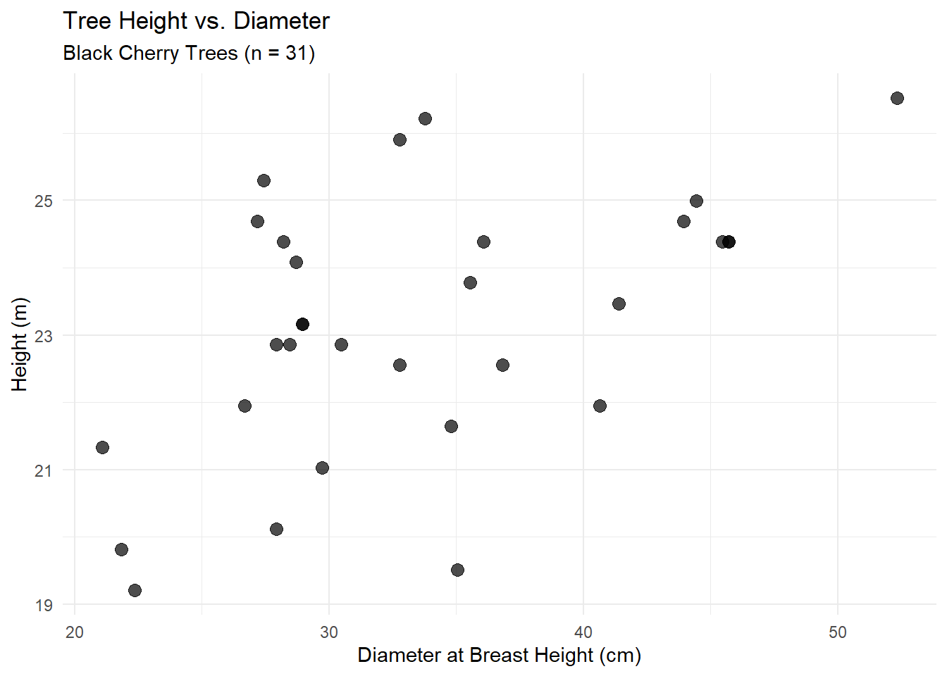
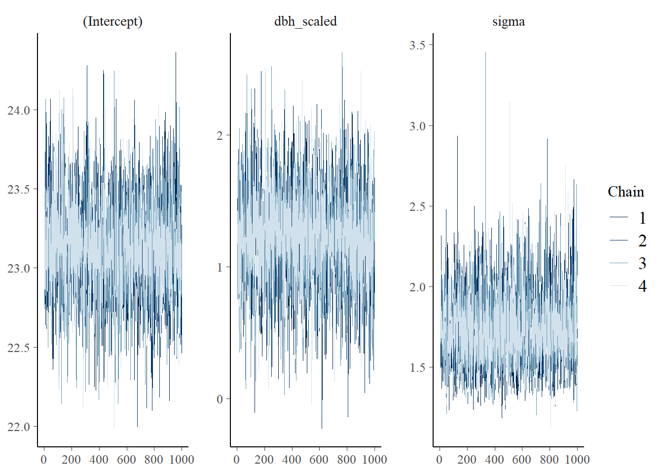
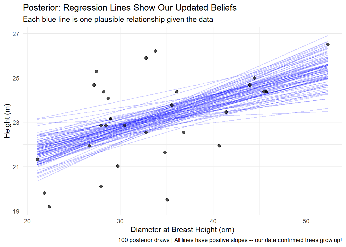
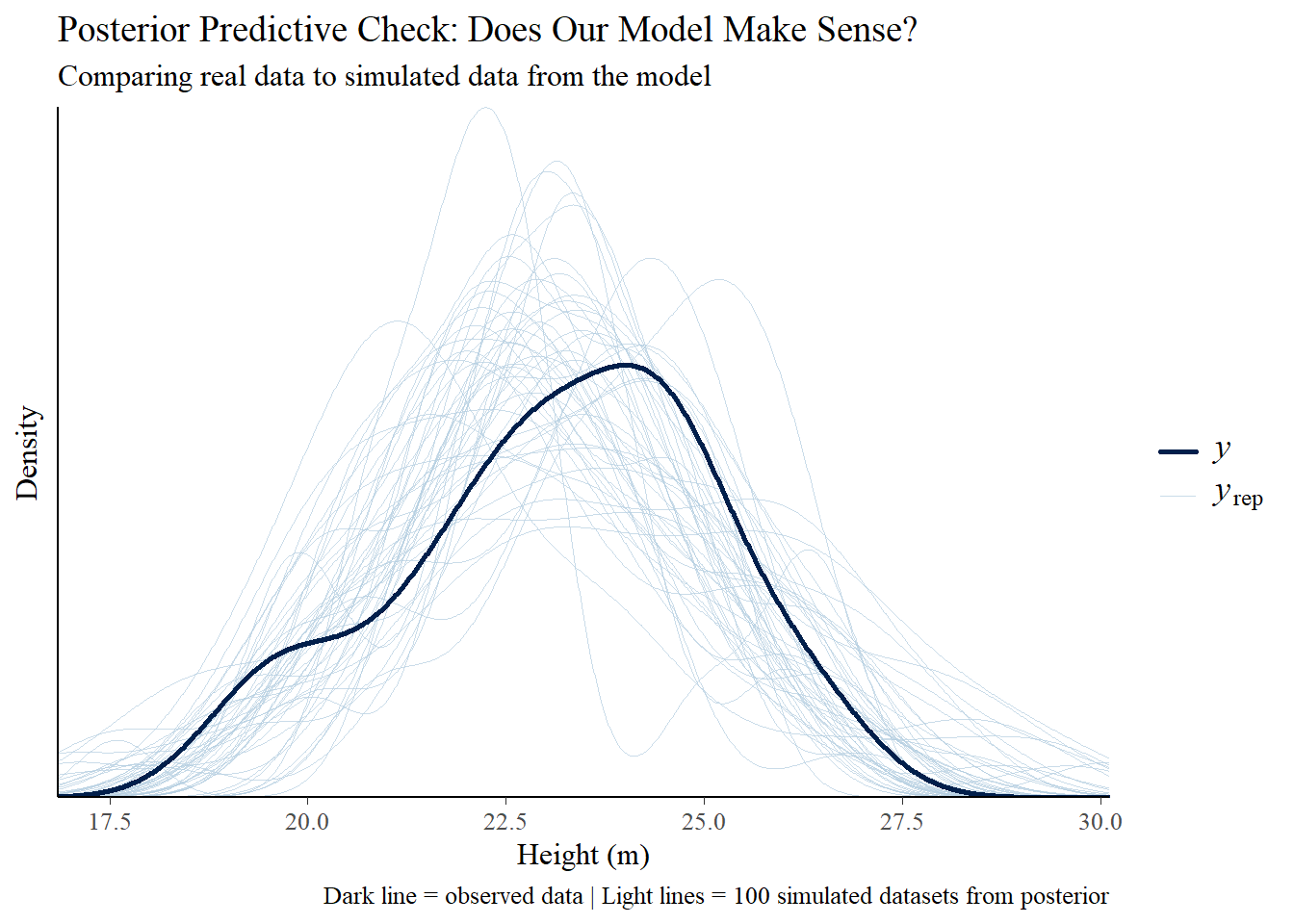
A Bayesian framework handles this the same way we analyzed tree height-diameter relationships earlier in this post: treat each uncertain input as a probability distribution, sample from all distributions simultaneously, and propagate uncertainty through the economic calculation. Instead of running the analysis once with fixed assumptions, you run it thousands of times, each time drawing different combinations of deployment rates, costs, gains, and market conditions from their respective distributions.

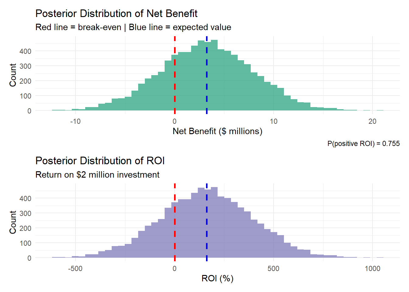
The result isn’t a single number but a full probability distribution of outcomes. Instead of “Expected NPV = $7.4M,” you get probability statements that directly answer the business question: “There’s a 73% chance of positive returns, a 45% chance NPV exceeds $5M, and an 8% chance of losses over $2M.” This directly answers the business question: “What’s the probability this investment pays off given everything we’re uncertain about?”

Schreiber & Thomas (2017) key insight makes it even more important: Deployment area matters as much as genetic gain. In Bayesian terms: If you can control deployment (reduce its uncertainty), you dramatically improve the probability distribution of returns. A company that commits to 20% deployment with high confidence has much better odds than one hoping for 15% but uncertain about achieving it.

Why This Matters

Forest companies face compound business uncertainty when evaluating long-term investments:

Operational uncertainties:

• Can we realistically achieve 15-20% deployment across diverse FMA areas?
• Will field crews consistently plant improved stock rather than wild seed?
• How do deployment logistics vary by terrain and access?

Financial uncertainties:

• Will breeding program costs stay manageable over decades?
• What will improved seedling costs be as production scales?
• How sensitive are returns to discount rate assumptions?

Biological uncertainties:

• Will 2.3% recognized gains translate to actual field performance?
• How much site-to-site variation should we expect?
• Will climate change affect genetic gain realization?

Market uncertainties:

• What will stumpage fees and lumber prices be over 20-year FMP cycles?
• How do mill closures or expansions affect our timber allocation?

This is where Bayesian inference provides clarity. Standard economic models analyze scenarios independently: “If deployment = 15% and costs = $3M and gains = 2.3%, then NPV = $7.4M.”

Bayesian models integrate across all uncertainties simultaneously: “Accounting for realistic uncertainty in deployment (10-25%), costs ($2-6M), gain realization (1.8-2.8%), and markets, there’s a 73% probability of positive NPV and a 45% probability NPV exceeds $5M.”

The critical insight: When only 3 of 7 companies proceed, it suggests the others looked at compound uncertainty and concluded the probability of success was too low. A Bayesian framework makes that reasoning explicit and quantifiable.

Moreover, it identifies which uncertainties matter most. If deployment rate is the dominant factor (as Schreiber & Thomas (2017) suggest), companies can focus on operational commitments that reduce deployment uncertainty rather than waiting for higher genetic gains. A company that can guarantee 20% deployment with high confidence faces much better odds than one hoping for 25% genetic gains that regulators may not recognize.

The Bayesian workflow we’ve demonstrated – specify priors, update with data, propagate uncertainty, make probability statements – applies directly to these multi-million dollar, multi-decade investment decisions where numerous uncertainties compound.

The gap between 2.3% recognized gains and 10-25% demonstrated gains creates a difficult business problem:

• small recognized gains mean economics are marginal, and
• compound uncertainties make outcomes unpredictable.

Only 3 of 7 Alberta programs found the risk-reward balance favorable. Quantifying probability of success under compound uncertainty – rather than analyzing scenarios independently – is exactly where Bayesian methods add value for complex, long-term business decisions.

Key Takeaways: From Seed Germination to Tree Improvement to Business Decisions

The Journey We’ve Taken

Over this three-post series, we’ve built a complete understanding of statistical inference:

Post 1 (Frequentist Foundations): We learned that frequentist inference is about procedures with long-run error rates. Confidence intervals describe what happens across hypothetical repetitions. P-values measure compatibility with null models. These tools are powerful when you want known error rates for repeated decisions.

Post 2 (Bayesian Foundations): We shifted to thinking about parameters as random variables representing our uncertainty. We learned that Bayesian inference naturally handles sequential learning, allows direct probability statements, and makes assumptions explicit through priors. The seed germination example showed these principles in action for a single parameter.

Post 3 (This Post): We scaled those principles to multiple parameters without changing the fundamental logic. Tree height regression used the same workflow: specify priors, check if they’re sensible, update with data, validate the model, make probabilistic predictions. The tree improvement example showed how this framework naturally handles real business decisions under uncertainty.

Core Principles That Carry Forward

1. Prior choice is critical but not mysterious

• Don’t use flat priors – they allow nonsense
• Use weakly informative priors that encode basic domain knowledge
• Always conduct prior predictive checks to validate your choices
• Your priors are assumptions made explicit, not a source of bias

2. Probability statements answer real questions

• “P(β > 0) = 0.98” directly answers “Is the effect positive?”
• “P(ROI > 0) = 0.85” directly answers “Will this investment pay off?”
• No need to translate between p-values and practical meaning

3. Uncertainty propagates through all calculations

• From parameter posteriors → to predictions → to economic outcomes
• This prevents false precision and enables realistic planning
• Point estimates hide critical information that full distributions reveal

4. The Bayesian workflow is consistent

1. Specify priors (encode domain knowledge)
2. Check priors (prior predictive checks)
3. Fit model (MCMC sampling)
4. Check convergence (Rhat, ESS, trace plots)
5. Validate model (posterior predictive checks)
6. Make inferences (probability statements)
7. Make predictions (full uncertainty)

5. Model checking is essential

• Prior predictive checks prevent nonsense inputs
• Posterior predictive checks catch model failures
• Diagnostic plots reveal computational problems
• Bad models give unreliable answers – always validate

What Changes and What Doesn’t

From 1 parameter to many:

• ✓ Same conceptual framework
• ✓ Same workflow steps
• ✓ Same interpretation of credible intervals
• ✗ More complex prior specification (but same principles)
• ✗ More computationally demanding (but MCMC handles it)
• ✗ More difficult visualization (but 2D plots of key relationships work)

From simple models to complex ones:

• The principles in this series extend to hierarchical models, time series, spatial statistics, and more
• Complexity grows in implementation, not in conceptual foundation
• If you understand updating beliefs about germination rates, you understand Bayesian inference

Practical Wisdom

When Bayesian methods shine:

• Making sequential decisions (examine data as it arrives)
• Quantifying probability of specific outcomes (P(effect > threshold))
• Incorporating prior knowledge from previous studies
• Communicating uncertainty to non-statisticians
• Small sample sizes where prior information helps

When to be cautious:

• Prior specification requires thought – no autopilot
• Computational demands can be substantial
• Different analysts with different priors may disagree (but so will frequentist analysts with different analysis choices)
• Skeptical audiences may question prior choices (though the same audiences accept arbitrary $\alpha$-levels)

The bottom line:

Both frequentist and Bayesian frameworks are legitimate approaches to statistical inference. They answer different questions and suit different contexts. The frequentist approach in Post 1 remains widely used, well-understood, and appropriate for many scientific questions. The Bayesian approach offers advantages for decision-making under uncertainty, sequential learning, and direct quantification of what we want to know.

The shift from thinking about procedures to thinking about beliefs is the essence of Bayesian inference. Once you internalize this shift – as we’ve done across three posts from seeds to trees – you can apply the same reasoning to arbitrarily complex models.

The real power isn’t in the fancy mathematics or the MCMC algorithms. It’s in the conceptual clarity of saying “Here’s what I believed before, here’s what I observed, here’s what I believe now, and here’s the probability of what I care about.”

That’s Bayesian inference. You already know how to think this way – we’ve just given you the mathematical tools to do it rigorously.

References

Galton, F. (1886). Regression towards mediocrity in hereditary stature. The Journal of the Anthropological Institute of Great Britain and Ireland, 15, 246–263. https://doi.org/10.2307/2841583

Pearson, K. (1896). Mathematical contributions to the theory of evolution.—III. Regression, heredity, and panmixia. Philosophical Transactions of the Royal Society of London. Series A, 187, 253–318. https://doi.org/10.1098/rsta.1896.0007

Schreiber, S. G., & Thomas, B. R. (2017). Forest industry investment in tree improvement—a wise business decision or a bottomless pit? Answers from a new tree improvement valuation model for Alberta, Canada. The Forestry Chronicle, 93(1), 38–43. https://doi.org/10.5558/tfc2017-009